Intro
The traveling salesperson is a classic computer science problem, for which there are many, many extensions to express different complexities. I’m learning a lot about the types of algorithms employed to solve these, so I thought it’d be good to write-up my learnings and take you dear reader along for the ride.
So, what’s the traveling salesperson?
Imagine you are a salesperson, taking your wares from city to city and selling them to the locals. Once they’ve bought their fill, you move on to the next city. Ideally you wouldn’t visit the same one again for a while, as you’ve already sated the needs of the populace and traveling itself is expensive, both in terms of time and fuel. Oh, and you’ll obviously want to end up at home, so you’ll need to make sure you return where you started. Simple!
A more condensed version of this might be:
Given a set of $N$ nodes and a starting point $n_i$ for $n \in N$, find the shortest path $P$ that visits all nodes at least once, and terminates at $n_i$.
There are many approaches to solve this problem, which is what this series will look at, but we’ll start with the simplest possible as a means of introducing concept, the Random Solution.
The Random Solution
It really cannot get more simple than this, given a set of cities to visit, put them in a random order! Done.
To do so however, we’ll need an algorithm to shuffle an array without bias:
/**
 * Fisher-Yates Shuffle.
 */
const shuffle = (arr: Array<any>) => {
  const shuffledArray = [...arr];
  let currentIndex = arr.length;
  let randomIndex = 0;

  while (currentIndex != 0) {
    randomIndex = Math.floor(Math.random() * currentIndex);
    currentIndex--;

    [shuffledArray[currentIndex], shuffledArray[randomIndex]] = [
      shuffledArray[randomIndex],
      shuffledArray[currentIndex],
    ];
  }

  return shuffledArray;
};
and then some representation of our problem space to act upon:
// Domain entities

class City {
  x: number;
  y: number;

  ...
}

class Trip {
  cities: City[];
  distance: number;

  ...
}

// Algorithm application

interface Move {
  /**
   * Mutate the solution, moving to a new state.
   */
  apply: (solution: Solution) => Solution;
}

class Solution {
  nodes: Cities[];
  trip: Trip;

  ...
}
(The full code for this post can be found here.)
So, let’s go over these concepts briefly. We’ve identified two aspects of our problem domain that we need to model, a City and a Trip, with the trip being a collection of cities that we’re visiting. On the other side, we have some aspects of our Solution Domain, a Move and a Solution. As we know that there are many different ways to visit a set of cities ($N!$ in fact), we’ll need a representation of a given solution and the ability to compare one solution to another, to see which is better. The Move on the other hand, is responsible for “moving” from one Solution, to another. This is a core aspect of what we’ll see in later posts, so it’s important to get the ground work in now.
So, back to comparing one solution to another. That’s the job of the Objective Function. This is a function who’s value is to be minimized or maximized over a set of solutions, to determine which is better. What do you just depends on the problem. If you’re trying to plan deliveries, then you might want seek maximizing the number of deliveries you complete. If you’re deciding recipes, you might want to minimize the amount of food that spoils.
If we were to create a graph of different solutions against an objective function, it might look like the figure below:
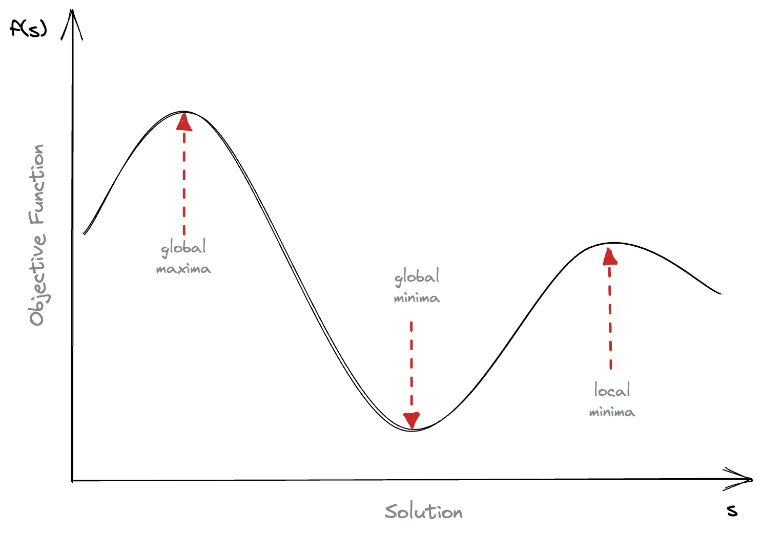
You’ll notice that there is a minima, a local maxima, and a global maxima. We’ll see later in later posts that detecting local minima / maxima is impossible, and accounting for them leads to some interesting algorithm design!
In our case, the objective function is quite simple: given a valid solution, how far does it travel? And when we compare one to another, we can check which is better by seeing which one travels the least. (This is so simple in fact, that you’ll notice that this is already present on our Trip entity.), Thus we can express our optimal solution as:
But, as we don’t intend on evolving the solution just yet though, we’ll just show the cost.
Below, it an output of the very beginning of our problem. The problem set I’ve chosen is known as ATT48, or the US State capitals. This is a very famous problem set, and thus the solution has been derived, but I’ve provided the ability for you to randomly try new ones.
After a few goes you might notice it:
- looks terrible
- does not perform very well
This is because you’re essentially throwing a deck of cards into the air, and hoping that they all land in order again. To put that into perspective your chances of doing so are $48! = 1.2 \times 10^{61}$, while there are only $10^{56}$ atoms in our solar system.
There must be a better way, and there is.
In the next post.